Entropy value method
The entropy value method is highly regarded for its objectivity and scientific rigor in dynamic comprehensive evaluations. Its core principle involves utilizing the information entropy of each index to determine its weight, and then calculating the comprehensive evaluation result via a weighted average. This method involves several key steps:
To address the issue of inconsistent measurement units among indicators, which could skew comparisons, the evaluation index data for DF and RSD must first undergo standardization. This process adjusts the scale of the indicators to a uniform metric, mitigating potential scale-related discrepancies. The standardization formulas for positive and negative indicators are as follows:
$$ {\text{Positive indicators}}:r_{ij} = \frac{{a_{ij} – \min (a_{ij} )}}{{\max (a_{ij} ) – \min (a_{ij} )}} $$
(1)
$$ {\text{Negative indicators}}:r_{ij} = \frac{{\max (a_{ij} ) – a_{ij} }}{{\max (a_{ij} ) – \min (a_{ij} )}} $$
(2)
where \(a_{ij}\) represents the original value of the indicator, while \(r_{ij}\) signifies the standardized, dimensionless value. The terms max(\(a_{ij}\)) and min(\(a_{ij}\)) denote the maximum and minimum values of the indicator \(j\) across all entities being evaluated, respectively. Following standardization, the entropy weight method is employed to ascertain the weight of each indicator, enhancing the accuracy of the comprehensive evaluation. The comprehensive development index for each system is then computed using the formula:
$$ U_{i} = \sum\limits_{j = 1}^{n} {w_{j} r_{ij} } $$
(3)
where \(U_{i}\) denotes the comprehensive development level of the system, \(w_{j}\) represents the weight of indicator \(j\), and \(n\) is the total number of indicators within the system. This approach ensures that the comprehensive index reflects the relative importance of each indicator, providing a nuanced and balanced assessment of the development level of each system.
Dual-system coupling coordination model
In physics, the concept of coupling describes how two or more systems interact and influence each other. The CCD model quantifies the level of coordination between different systems. It has been widely applied across various disciplines, including economic, social, and environmental development. In economics, this model is primarily used to analyze the coordinated development levels among multiple systems, such as the interaction between the ecological environment, economy, and human society. For instance, it measures the interplay between ecology and economy32,33. Furthermore, it has been extensively utilized in research on green finance34,35 and sustainable development36.
This paper introduces the CCD model to assess the coupling and coordination between DF (\(U_{1}\)) and RSD (\(U_{2}\)).The model aims to evaluate the coordination effects and the dynamic evolution of the relationship between DF (\(U_{1}\)) and RSD (\(U_{2}\)). The mathematical formulation of the model is as follows:
$$ C = \sqrt {\frac{{U_{1} \times U_{2} }}{{\left( {\frac{{U_{1} + U_{2} }}{2}} \right)^{2} }}} $$
(4)
$$ T = \frac{{U_{1} \times U_{2} }}{2} $$
(5)
$$ D = \sqrt {C \times T} $$
(6)
In these equations, \(U_{1}\) and \(U_{2}\) represent the respective levels of DF and RSD. \(C\) signifies the system’s harmonization level, with values ranging from 0 to 1, reflecting the extent of synergy between DF and RSD. \(T\) is the combined evaluation score of the two systems.\(D\) quantifies the overall coupling effect, also within a range of 0 to 1. A higher \(D\) value indicates a stronger coupling and a more synergistic relationship, promoting mutual and coordinated development between DF and RSD.
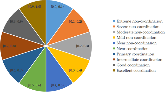
To depict the CCD between DF and RSD more vividly, this study adopts a classification scheme inspired by Hou et al.37, dividing the CCD into 10 distinct grades. These grades provide a nuanced view of the interaction dynamics, facilitating a deeper understanding of how these systems co-evolve and influence each other. The classification of these grades will be illustrated in Fig. 3, offering a detailed visual representation.
Kernel density estimation
This study utilizes the kernel density estimation method to examine the distributional dynamics and variation in the CCD between DF and RSD across six major city clusters in China. The kernel density estimation, a non-parametric way to estimate the probability density function of a random variable, is defined as follows:
$$ f(x) = \frac{1}{nh}\sum\limits_{i = 1}^{n} {K\left( {\frac{{\overline{x} – x_{i} }}{h}} \right)} $$
(7)
where \(K\) is the kernel function, \(X_{1} , \cdots X_{n}\) is the CCD of the cities in the sample, \(\overline{x}\) is the mean value, \(n\) is the number of sample observations, and \(h\) is the window width. The article selects the Gaussian kernel function with high-precision reading to estimate the dynamic distribution level of the CCD of DF and RSD of the six major city clusters, and its functional expression is:
$$ K(x) = \frac{1}{{\sqrt {2\pi } }}e^{{\left( { – \frac{{x^{2} }}{2}} \right)}} $$
(8)
Markov chains
Markov chains are employed to analyze the distribution and evolutionary trends of the CCD across different time frames and states, categorizing continuous values into discrete classes. Initially, a conventional Markov chain analysis dissects the internal trend characteristics of the system’s CCD. Here, the quartile method segments the CCD into four distinct levels: low, medium–low, medium–high, and high, based on their average values, facilitating the computation of the transition probability matrix. Subsequently, to incorporate spatial dynamics, a spatial Markov transition probability matrix (MTPX) is formulated following a spatial correlation assessment. Unlike the traditional Markov chain, the spatial Markov chain addresses the oversight of inter-regional interactions by integrating the concept of “spatial lag”. This approach involves calculating the weighted average attribute value of adjacent regions using a spatial weight matrix, thereby assessing the spatial lag condition of regional entities. This method, as Chen and Zhu38 note, enhances the analytical framework by considering the spatial dependencies and interactions among regions, offering a more comprehensive understanding of the CCD’s spatial and temporal evolution.
Convergence analysis
\(\sigma\)-convergence
To assess the convergence trends of the CCD between DF and RSD across six major city clusters in China, this study employs the coefficient of variation to perform σ-convergence analysis. This involves examining the temporal trend of the CCD’s coefficient of variation both for the entire sample and within each of the six city clusters, to determine if regional disparities are diminishing over time. The coefficient of variation is calculated using the following formula:
$$ CV_{it} = \frac{{\sigma_{it} }}{{\overline{D}_{it} }} = \frac{{\sqrt {\frac{1}{{m_{i} }}\sum\limits_{m = 1}^{{m_{i} }} {(D_{imt} – \overline{D}_{it} )^{2} } } }}{{\overline{D}_{it} }} $$
(9)
Here, \(\sigma_{it}\) represents the standard deviation of the CCD across the city clusters in year \(t\), \(D_{imt}\) denotes the coupling coordination level of the city \(m\), region \(i\) in year \(t\), \(m_{i}\) denotes the number of cities included in region \(i\), and \(\overline{D}_{it}\) denotes the average value of the CCD of all cities in region \(i\) and year \(t\).
\(\beta\)-convergence
In this study, \(\beta\)-convergence is utilized to explore the evolution of the CCD between DF and RSD across six major city clusters. \(\beta\)-convergence, stemming from neoclassical growth theory, is categorized into absolute and conditional \(\beta\)-convergence. The spatial correlation analysis conducted in this research indicates a substantial positive link between the DF and RSD coordination levels across these clusters. Conventional convergence theories often overlook the spatial interdependencies among regions. To address this gap, the current analysis incorporates an economic distance spatial weight matrix, enhancing the assessment of spatial convergence. Through rigorous testing, including Lagrange Multiplier (LM), Hausman, and Likelihood Ratio (LR) tests, the study opts for a two-way fixed-effects spatial Durbin model (SDM). This model is adept at evaluating both absolute and conditional \(\beta\)-convergence, providing a more nuanced understanding of how the CCD between DF and RSD evolves over time and space within the context of these city clusters. The SDM framework is specifically designed to capture the intricate spatial interactions, thereby offering a comprehensive analysis of convergence dynamics. The model is formulated as follows:
$$ \ln \left( {\frac{{q_{i,t + 1} }}{{q_{i,t} }}} \right) = \alpha + \beta \ln (q_{i,t} ) + \rho W_{ij} \ln \left( {\frac{{q_{i,t + 1} }}{{q_{i,t} }}} \right) + \gamma W_{ij} \ln (q_{i,t} ) + \mu_{i} + \eta_{t} + \varepsilon_{it} $$
(10)
$$ \begin{aligned} \ln \left( {\frac{{q_{i,t + 1} }}{{q_{i,t} }}} \right) = & \alpha + \beta \ln (q_{i,t} ) + \sum\limits_{z = 1}^{n} {\lambda_{z} X_{it} + } \rho W_{ij} \ln \left( {\frac{{q_{i,t + 1} }}{{q_{i,t} }}} \right) + \gamma_{1} W_{ij} \ln \left( {q_{i,t} } \right) \\ + \sum\limits_{z = 1}^{n} {\gamma_{2z} W_{ij} X_{it} } + \mu_{i} + \eta_{t} + \varepsilon_{it} \\ \end{aligned} $$
(11)
where \(q_{it}\) denotes the CCD between DF and RSD of city \(i\) in year \(t\), and \(\ln (\frac{{q_{i,t + 1} }}{{q_{i,t} }})\) denotes the growth rate , \(\beta\) is the convergence coefficient, if \(\beta < 0\) then it means that there is a convergence trend in the DF and RSD coupling coordination level across cities over time. Conversely, a positive \(\beta\) signifies divergence. The rate of convergence is \(\upsilon = – \ln (1 + \beta )/T\), \(T\) represents the duration of the study, with the half-way convergence period \(\tau = \ln (2)/\upsilon\). \(\rho\) is the spatial lag coefficient, and \(W_{ij}\) is the spatial weight matrix, here the economic distance matrix is selected as the spatial weight matrix, specifically using the GDP gap of each city as a measure of economic distance between cities. \(\mu_{i} ,\;\eta_{t} ,\;\varepsilon_{it}\) represent city-fixed effects, time-fixed effects, and random error terms, respectively. \(X_{it}\) is the selected control variables, referring to the existing literature39, the analysis framework of the factors influencing the CCD of DF and RSD is mainly constructed from five aspects: the level of economic growth, government intervention, financing constraints, software technology practitioners, and the level of informatization.


