Automatic classification of uveal melanoma response patterns following ruthenium-106 plaque brachytherapy using ultrasound images and deep convolutional neural network

Study workflow

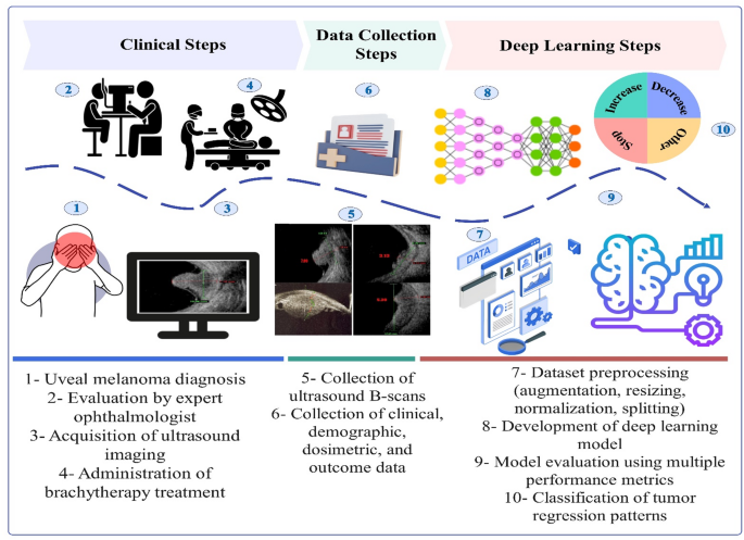
Figure 1 illustrates the complete workflow adopted in this study, encompassing clinical procedures, data collection, and DL implementation. The objective is to explore the feasibility and effectiveness of DL in predicting UM response patterns. The process begins with the identification of UM in patients (Step 1), followed by a clinical examination by an Ocular oncologist (Step 2). Ultrasound imaging is performed (Step 3), and plaque brachytherapy is administered by a multidisciplinary team of physicians and medical physicists (Step 4). B-scan ultrasound images are then collected (Step 5), along with clinical, demographic, dosimetric, and follow-up data (Step 6). These data are preprocessed through augmentation, resizing, normalization, and dataset splitting (Step 7), after which the DL model is developed (Step 8) and evaluated using standard performance metrics (Step 9). The final outcome is a multi-class prediction of UM response patterns, including increase, decrease, stop, and other categories (Step 10).

Study cohort

This retrospective, single-center study was conducted at the Eye Research Center. Due to the retrospective nature of the study, the Ethics Committee of IUMS (IR.IUMS.FMD. REC.1402.417) waived the need to obtain informed consent and approved the experiments. All methods were performed in accordance with the relevant guidelines and regulations. The study population included adult patients clinically diagnosed with UM between July 2017 and 2022 who underwent treatment with ruthenium-106 plaque brachytherapy. The exclusion criteria included: (1) age under 18, (2) prior treatment with therapies other than ruthenium-106 plaque brachytherapy, (3) follow-up duration of less than two years, (4) presence of metastatic disease at diagnosis, and (5) patients of other nationalities.

B-Mode ultrasound images of 192 patients were collected at the time of uveal melanoma diagnosis and before the start of brachytherapy treatment. Each patient had at least two images in both transverse and longitudinal views at the time of diagnosis, so a total of 661 images were collected. Each patient had at least 2 years of follow-up, so the ocular oncologist labeled the patients’ images into four groups in terms of response pattern, increase, decrease, stop, and other, based on the response to treatment of the mass during follow-up sessions. Additionally, US images were independently interpreted and reported by two board-certified ophthalmologists specializing in ocular oncology, each with a minimum of 10 years of experience.

Response patterns in intraocular melanoma post-brachytherapy

Patients were treated with ruthenium 106 (Eckert & Ziegler BEBIG company, Berlin, Germany) plaques to deliver the appropriate dose to the apex and base of the tumor. Three plaque types were utilized: round (CCA, CCB, and CGD), notch (COB), and Ciliary body (CIA). An experienced medical physicist oversaw the dosimetry process, ensuring accurate dose delivery based on the activity and half-life of the ruthenium-106 plaques. The physicist also documented the dosimetry reports for each treatment. An ocular oncologist measured tumor thickness and the largest basal diameter (LBD). Tumor thickness was assessed from the inner scleral surface to the tumor apex along two meridians: one along the LBD and another perpendicular to it. Representative digitized scans were prospectively stored during each diagnostic and follow-up visit. We tracked the changes in tumor thickness and the LBD over time and classified tumor response patterns according to Abramson et al.²⁷, using four main categories: D (decrease; a progressive reduction in thickness by at least 15% post-brachytherapy), S (stable; less than 15% change in thickness), I (increase; a progressive increase in thickness by at least 15%), and Others²⁷. The Others category was further divided into five subtypes: DS (decrease followed by stability), DI (decrease followed by increase), ID (increase followed by decrease), SD (stability followed by decrease), and zigzag (alternating measurements with no clear trend). A total of 661 images were collected from 192 patients with intraocular melanoma before the beginning of treatment. All images were acquired by a single operator and independently interpreted by two ophthalmologists, each with over ten years of experience in plaque radiotherapy for UM. As illustrated in Fig. 2, B-Mode US images of four different patients with Decrease, Other, Stop, and Increase response pattern at the time of diagnosis (a1, a2, a3, and a4), one year (b1, b2, b3, and b4), and two years (c1, c2, c3, and c4) post-treatment with Ru-106 plaque brachytherapy.

Data preprocessing

All US images were obtained in JPEG format from the US imaging databases. A 5-fold cross-validation (CV) approach was applied to split the dataset, using 80% for training and 20% for testing in each fold. To address the class imbalance, oversampling was performed by applying horizontal flipping, rotation, shifting, scaling, and brightness/contrast adjustments. This process ensured that all classes contained equal number of images.

Before augmentation, the Increase group contained 36 images, the Decrease group had 336 images, the Stop group included 125 images, and the Other group consisted of 164 images, and after augmentation increased to 3966 images. Before model training, images were resized to 224 × 224 pixels to match input requirements. Normalization was applied using a mean of [0.485, 0.456, 0.406] and a standard deviation of [0.229, 0.224, 0.225] and conversion to tensor format, ensuring consistency with pre-trained models.

Deep learning model construction

Two convolutional neural network architectures, DenseNet121 and ResNet34, were utilized as the backbone models for image multi-class classification. These architectures were chosen due to their proven ability to perform well in image classification tasks while maintaining reasonable computational efficiency. Both models were initialized with random weights (weights = None) and trained under identical conditions to ensure a fair comparison.

DenseNet121 is composed of five dense blocks organized across three transition levels, with each block containing multiple convolutional layers followed by a max-pooling operation. The architecture leverages dense connectivity, where each layer receives input from all preceding layers, promoting feature reuse and mitigating the vanishing gradient problem. The final output, after global average pooling, is passed through a series of fully connected layers, followed by a dropout layer (p = 0.4) tailored for four-class classification.

ResNet34, on the other hand, is structured around residual learning, consisting of an initial convolutional layer followed by four stages of residual blocks, each incorporating identity shortcut connections. These skip connections allow gradients to propagate more effectively during training, enabling deeper network architectures without degradation in performance. In the case of ResNet34, the final fully connected layer was similarly modified to include a linear transformation and a dropout layer with the same probability of performing four-class classification. Both models were trained using 2D ultrasound images and the corresponding ground truth labels provided in the dataset. Input images were resized to 224 × 224 pixels and normalized using ImageNet statistics.

Training was performed using stochastic gradient descent (SGD) with a learning rate of 0.001, momentum of 0.9, and weight decay of 1e-4. The loss function used was cross-entropy with label smoothing (ε = 0.1). A five-fold CV approach was implemented to ensure robustness. Training was conducted over 200 epochs, where each epoch involved forward propagation, loss computation, gradient backpropagation, and weight updates.

Ablation study

To evaluate the contribution of individual components within the model architecture and training strategy, a series of ablation experiments were performed. Each experiment involved modifying a specific element while keeping all other parameters constant to isolate its impact on model performance. Since DenseNet121 outperformed ResNet34, all three ablation scenarios were conducted exclusively for DenseNet121: (1) initializing the network with pre-trained ImageNet weights, (2) reducing the batch size to 16, and (3) removing dropout layers from the architecture. The results of these experiments provided insights into the sensitivity of the model to various training configurations and optimization strategies.

Performance evaluation

The model performance is validated on the test set after each epoch, with key performance metrics logged for analysis. These metrics provide a comprehensive assessment of the model’s performance:

• Confusion Matrix, Accuracy, Recall (Sensitivity), Precision, F1 Score, ROC Curve, and AUC (area under the curve).

• Macro average computes the AUC for each class individually and then averages the results. This approach treats all classes equally, regardless of their frequency in the dataset.

• Micro average aggregates the contributions of all classes to compute a global AUC score.

These averages provide a broader view of model performance across all classes.

• Cohen’s Kappa Coefficient: The Kappa coefficient evaluates agreement between predicted and actual classifications while accounting for chance agreement. It ranges from − 1 to 1, where a Kappa of 1 indicates perfect agreement, 0 suggests no agreement beyond chance, and values below 0 reflect worse-than-random performance, indicating poor model reliability. P-values < 0.05 were considered statistically significant.

These metrics together offer a robust evaluation of model performance across multiple dimensions. To estimate the statistical uncertainty associated with each metric, 95% confidence intervals (CIs) were calculated using bootstrap resampling with 1,000 iterations. In each iteration, the test set was resampled with replacement, and metrics such as accuracy, F1-score, and AUC were recalculated. The resulting metric distributions were then used to derive percentile-based 95% CIs. To assess whether the differences in AUC between models were statistically significant, DeLong’s test was applied.

Ethics approval

The Ethics Committee of IUMS waived the requirement for ethical approval (IR.IUMS.FMD. REC.1402.417).